Phylogenetics III
Bayesian phylogenetics
Public Health Modeling Unit
2025-08-19
Barney Isaksen Potter
Series overview
Trees, tree likelihoods, and models of evolution
Rate heterogeneity and maximum likelihood
Bayesian phylogenetics, Markov chain Monte Carlo, and summary trees
Phylogeography and Kingman's coalescent
please bear with me, timing may be off
Thank you Philippe
"the global workhorse of genomic epidemiology"
One Tree to rule them all, One Tree to find them, One Tree to bring them all and in the darkness bind them
The (maximum likelihood) method we've learned so far gets a single tree
The one it finds is likely not the "best"
Are we doing a good job of reporting a single tree?
ML produces a "point estimate" or a single inference of parameters:
Tree
Branch lengths
Model parameters
Frequentist philosophy
Probabilities refer to the outcome of experiments (i.e. data)
Probabilities are objectively real in the same way that physical objects are real
"Likelihood" referes to the degree to which data support a hypothesis
Frequentist = ML
Probabilities cannot exist without data/experiments
Bayesian philosophy
BOTH data and model parameters are described by probabilities
Probability represents the degree to which we believe a hypothesis
Hypotheses can have probabilities in the absence of data
We already know things about reality
We are interested in quantifying uncertainty
Bayesian inference
First, we will discuss Bayesian inference generally
Fundamentals of Bayesian inference
Bayesian inference produces a posterior probability distribution instead of a single MLE
The posterior combines information from both data and prior knowledge
Each parameter in the model has a prior probability distribution representing known knowledge about that parameter
Combine prior knowledge with data
Create a posterior distribution
Distribuion (rather than point estimate) helps us quantify uncertainty
"Human heights follow a uniform (flat) distribution between 1 angstrom and the width of the universe."
Technically proper, but extremely uninformative prior means that the data provide all the information
"Human heights follow a uniform (flat) distribution between 1 angstrom and the width of the universe."
Technically proper, but extremely uninformative prior means that the data provide all the information
"Human heights follow a uniform (flat) distribution between 1 angstrom and the width of the universe."
Technically proper, but extremely uninformative prior means that the data provide all the information
"Human heights follow a uniform (flat) distribution between 1 angstrom and the width of the universe."
Technically proper, but extremely uninformative prior means that the data provide all the information
"Human heights follow a normal distribution with mean 170cm and standard deviation 5cm."
We can wikipedia some facts about humans
Same data as before
Now there are two distributions that we need to combine
"Human heights follow a normal distribution with mean 170cm and standard deviation 5cm."
Only two data -> posterior is similar to the prior
Lots of data -> posterior is driven by the data. Maybe we aren't sampling from all humans
How can observing data (X ) change our belief in a hypothesis ($\theta$ )?
Talk through posterior, model, prior, then marginal
How can observing data (X ) change our belief in a hypothesis
($\theta$ )?
This term is a constant, represents the probability of the data if we integrate over all possible hypotheses
How can observing data (X ) change our belief in a hypothesis
($\theta$ )?
This term is a constant, represents the probability of the data if we integrate over all possible hypotheses
How can observing data (X ) change our belief in a hypothesis
($\theta$ )?
This term is a constant, represents the probability of the data if we integrate over all possible hypotheses
How can observing data (X ) change our belief in a hypothesis
($\theta$ )?
This term is a constant, represents the probability of the data if we integrate over all possible hypotheses
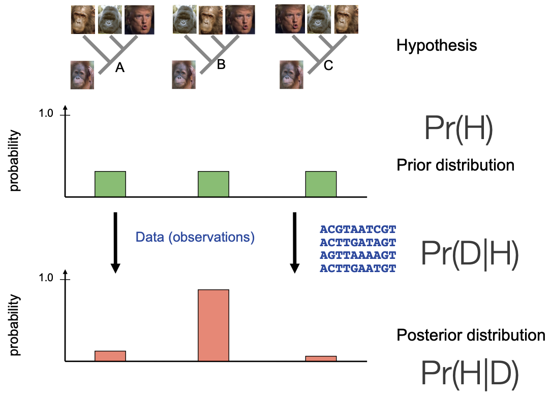
How can we apply this framework to phylogenetic inference?
We have multiple competing hypotheses for how four organisms could be related
No reason to favor one over the other -> uninformative prior
We apply data in the form of sequence data in tree likelihood calculations
We end up with aposterior distribution of trees that is informed by the data
\[
P(\theta|\textbf{X}) = \frac{P(\textbf{X} |\theta) \times P(\theta )}{P(\textbf{X})}
\]
We are now going to just change the symbols we use to fit our purpose
The posterior probability of a phylogenetic tree, $\tau$:
$\tau = $ phylogenetic hyopthesis (tree)
$\textbf{X} =$ genomic sequence data
Likelihood calculation
$\begingroup \color{darkmagenta} \tau = \text{tree topology} \endgroup, \begingroup \color{darkblue} \nu = \text{branch lengths} \endgroup, \atop \begingroup \color{mediumseagreen} \Theta = \text{model parameters} \endgroup, i \in \text{sites in genome}$
Let's break down the first term
Expand the likelihood to consist of four parts
Tree topology (shape)
Branch lengths
Model parameters
Data observations at each of the N sites in the genome
Because we assume sites are independent we can take the product of probabilities across all N sites
Calculated the same way as in ML
Prior calculation
$\begingroup \color{crimson} B(s) = \text{number of possible topologies} \endgroup$
Uniform prior on tree shapes
If we have other parameters, they will also have priors that get multiplied here
Marginal term calculation
To calculate this we need to sum the density across every possible tree...
Recall: we are calculating the average probability of the data across all possible hypotheses.
This means we are essentially performing a discrete integral over every possible tree topology.
... but tree topology space is too big!
\[\tiny
\begin{array}{cc}
\text{Num.~taxa} & \text{Num.~topologies:} \begingroup \color{crimson} B(s) \endgroup \\ \hline
1 & 1 \\
2 & 1 \\
3 & 3 \\
4 & 15 \\
5 & 105 \\
6 & 945 \\
7 & 10,395 \\
8 & 135,135 \\
9 & 2,027,025 \\
\vdots & \vdots \\
20 & 8,200,794,532,637,891,559,375 \\
\vdots & \vdots \\
769 & 3.753 \times 10^{2,110} \\
\end{array}
\]
This should be familiar already
Number of topologies scales superfactorially with number of taxa
Number is intractable for even relatively small datasets
8 sextillion: on the same order as the number of grains of sand or number of possible udoku grids
\[
3 \times 5 \times 7 \times \mathellipsis \times (2n-3)
=
\frac{(2n-3)!}{2^{n-1} \times (n-1)!}
\]
We derive this by considering, for each topology of n-1 taxa, how many places we could add a new branch along a prexisting one
Markov chain Monte Carlo (MCMC)
We need a clever algorithm to perform these computations
Markov chain Monte Carlo (MCMC) Sampling
Posterior probabilities are difficult to calculate analytically. However, we can sample values from the posterior distribution with a frequency proportional to thir posterior probability by using MCMC.
We can numerically approximate the full calculation by taking samples from the posterior distribution. If those samples are taken proportional to their posterior probability then we can summarize the samples to summarize the posterior.
Recall: ML optimization
ML uses a "hill climbing" algorithm to find the maximum likelihood, and only ever steps uphill. Downside: we don't know the shape of the distribution, and we may get caught in a local optimum
Recall: ML optimization
ML uses a "hill climbing" algorithm to find the maximum likelihood, and only ever steps uphill. Downside: we
don't know the shape of the distribution, and we may get caught in a local optimum
Recall: ML optimization
ML uses a "hill climbing" algorithm to find the maximum likelihood, and only ever steps uphill. Downside: we
don't know the shape of the distribution, and we may get caught in a local optimum
Recall: ML optimization
ML uses a "hill climbing" algorithm to find the maximum likelihood, and only ever steps uphill. Downside: we
don't know the shape of the distribution, and we may get caught in a local optimum
Recall: ML optimization
ML uses a "hill climbing" algorithm to find the maximum likelihood, and only ever steps uphill. Downside: we
don't know the shape of the distribution, and we may get caught in a local optimum
Recall: ML optimization
ML uses a "hill climbing" algorithm to find the maximum likelihood, and only ever steps uphill. Downside: we
don't know the shape of the distribution, and we may get caught in a local optimum
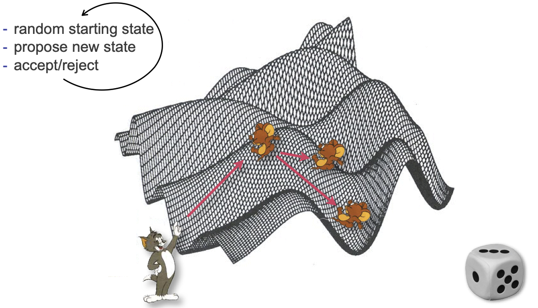
MCMC leverages randomness
Consider the black dots now
Use randomness cleverly to allow steps "downhill", in such a way that we end up with samples that cover the distribution proportional to its height
Green: we can have many steps downhill, though it is unlikely
Metropolis-hastings algorithm
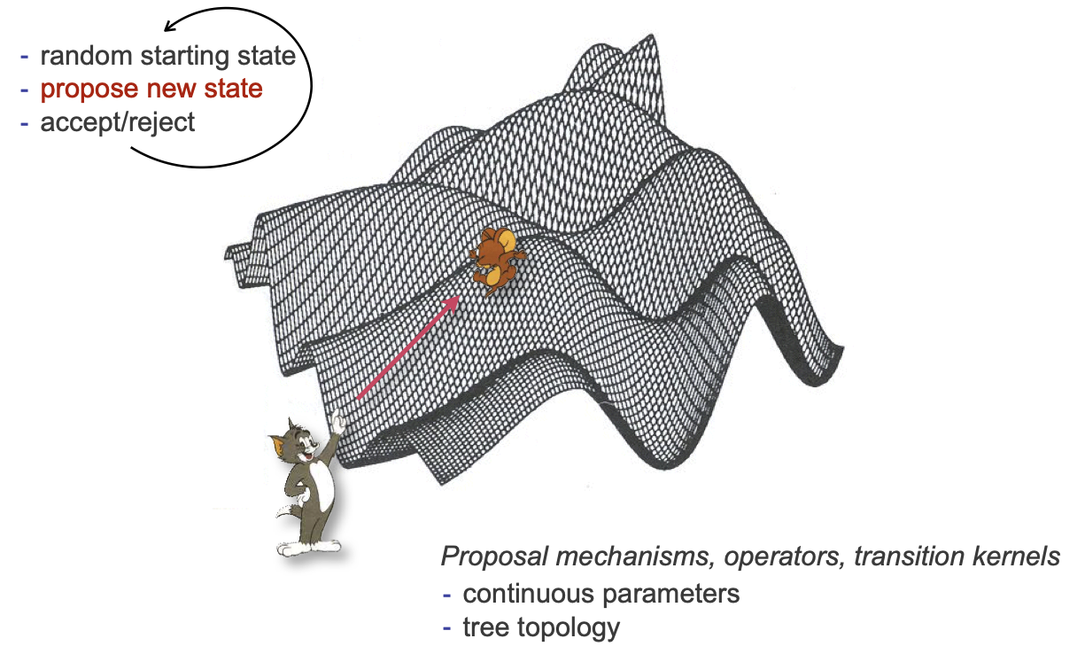
Core idea of the MH algorithm:
Start with a random state (calculate its likelihood)
Propose a random step from that state
Based on the likelihood at the new state, either accept or reject
Repeat (a lot)
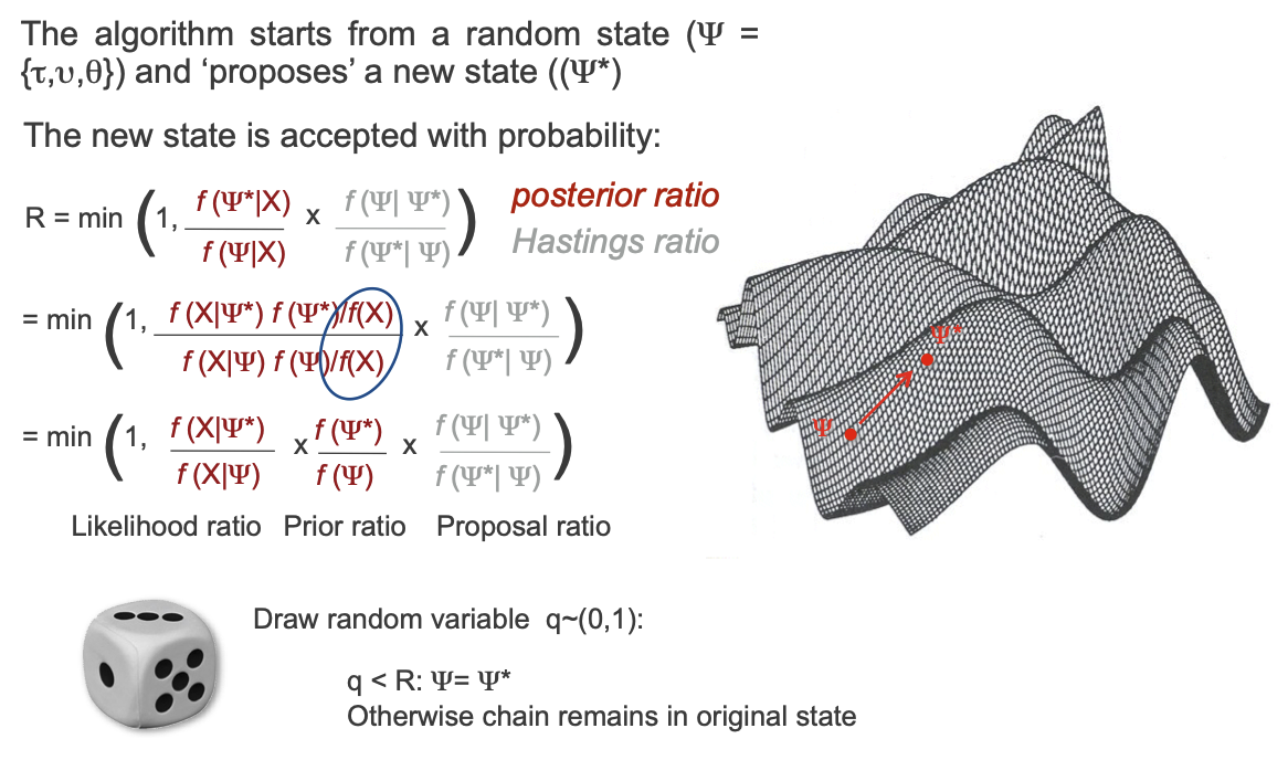
Recall: our state tau=tree, nu=branch lengths, Theta=model parameters
The algorithm proposes a new, modified state Psi star
Calculate a ratio R:
Ratio of posterior probabilities
Term "Hastings ratio" that accounts for potential asymmetry in proposals (ignore)
Expand posterior probabilities according to Bayes' theorem
Same problem as earlier, except that the marginal terms (B(s)) cancels out!
This is the crux of MCMC, because it allows us to never calculate the marginal term
The end result is a value between 0 and 1 that is proportional to the ratio of the likelihoods between Psi and Psi star
Generate a random number uniformly between 0 and 1
If that value is less than the ratio R, we accept the new proposal
Takeaway: we always take a step up, we often take small steps down, we rarely (but sometimes) take big steps down
Let's catch our breath for a minute
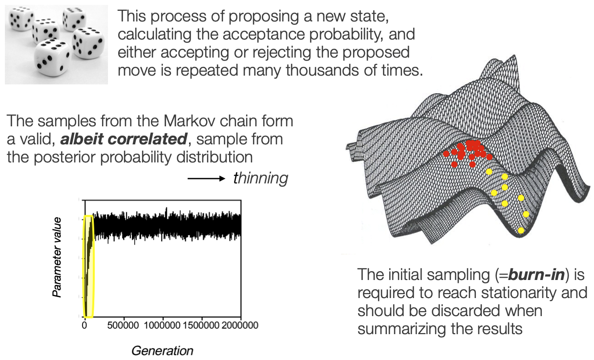
This process is repeated many many many times
All the samples that we keep describe the posterior distribution
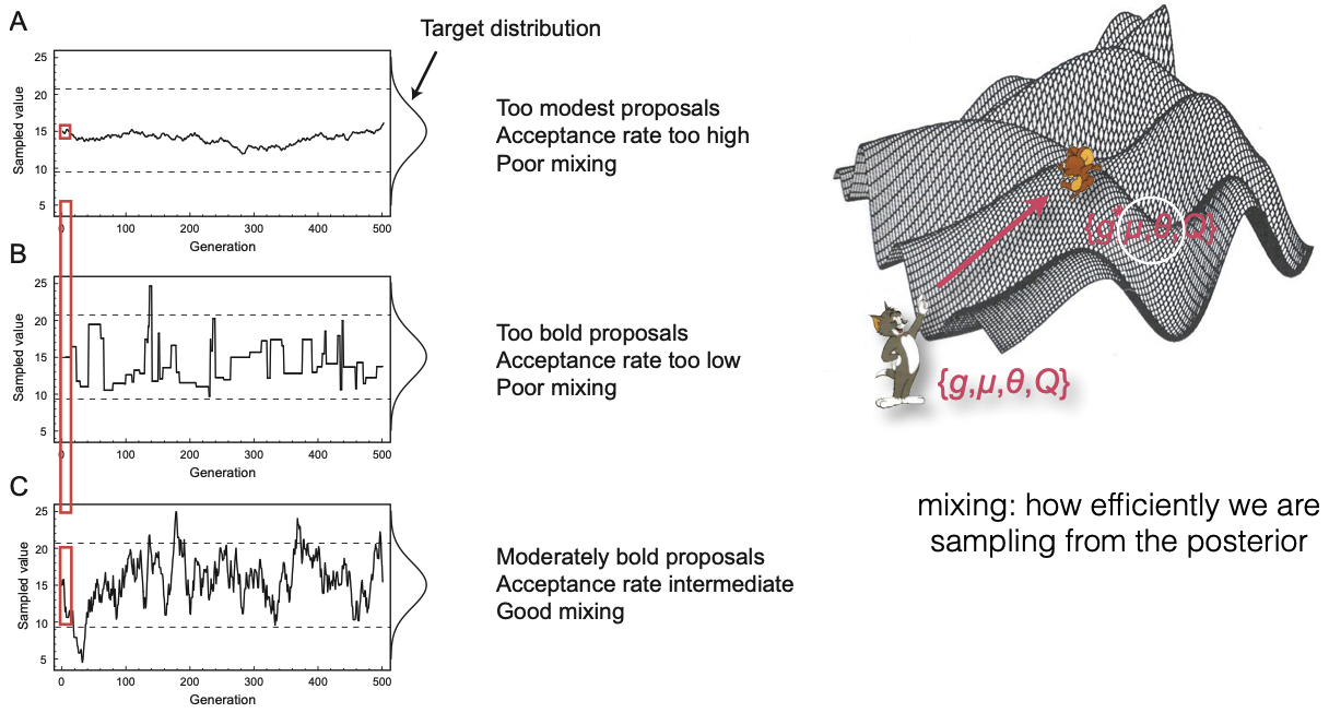
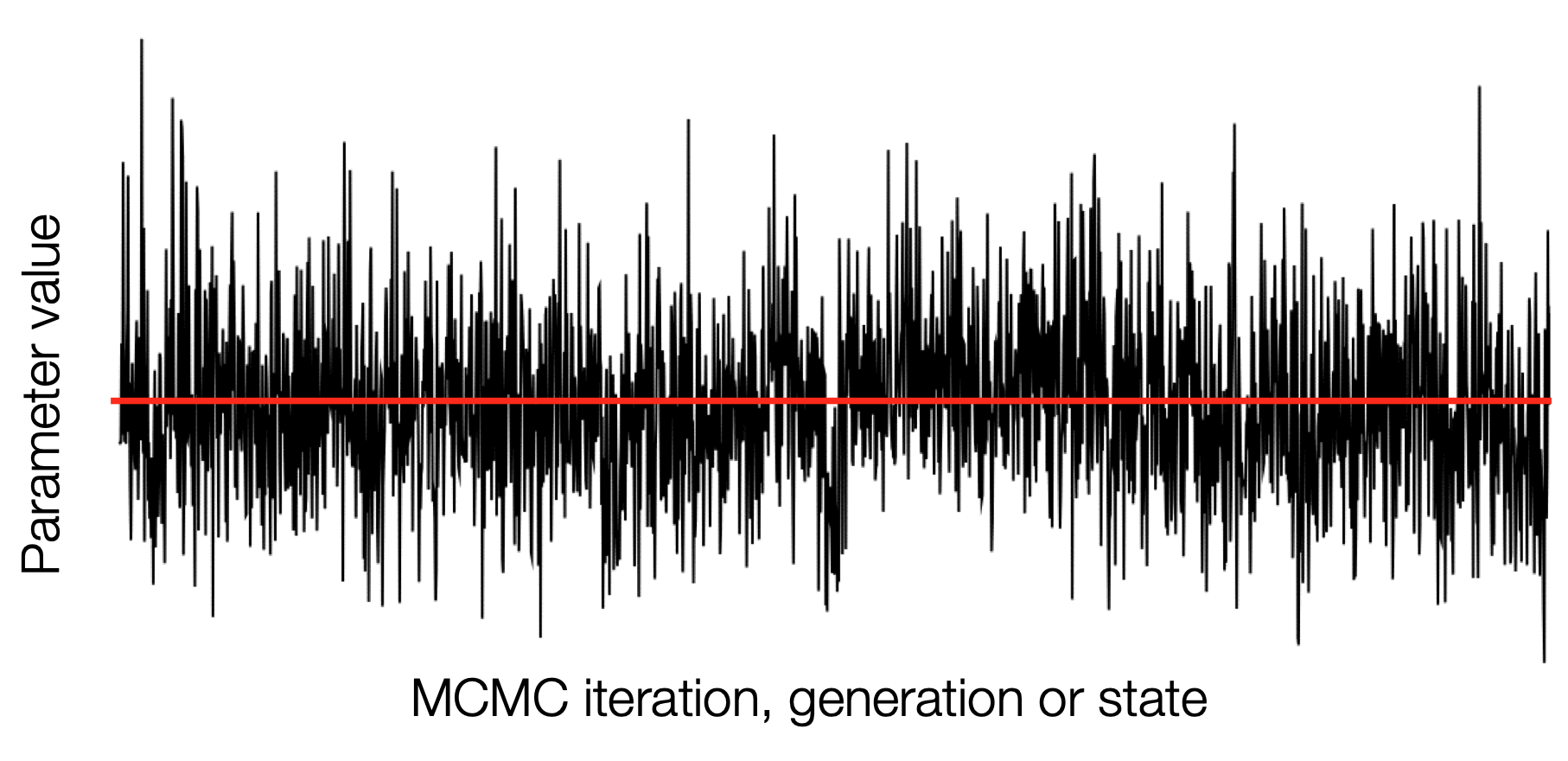
EXPLAIN the trace plot
apologize for no Tom and Jerry
ORIENT WITH THE INTERFACE
RandomWalkMH
normal
autoplay off
autoplay delay 500
animate proposal
walk through how it works for a few steps, then animate, then speed up
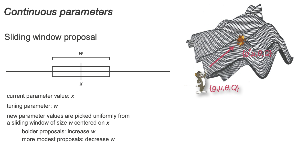
Now we can talk about how the new states get proposed. Many names, a couple major categories.
Operators
Many ways to make new continuous proposals
Simplest example: uniform pick from a window
Tuning prameters are useful!
Tuning and mixing
We use the word "mixing" to describe how efficiently we are sampling from the posterior
We can look at the acceptance rate for the operator to see if our proposals are good
mess with sigma on multimodal
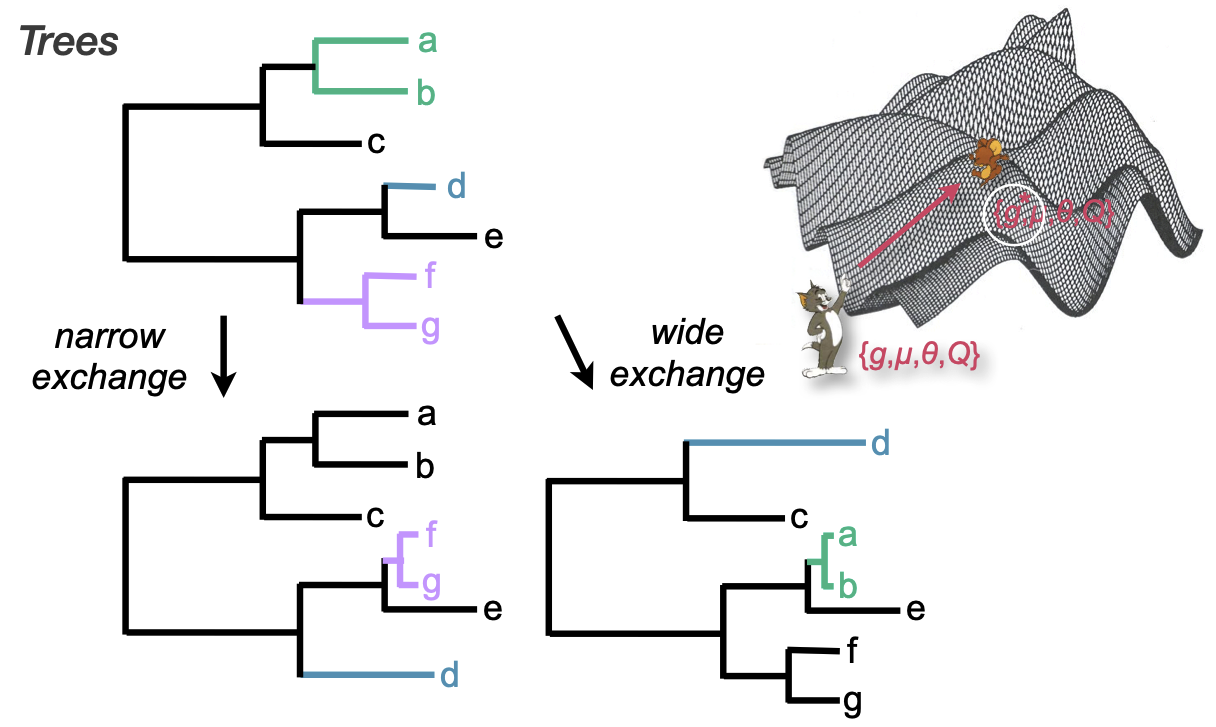
Operators on trees
Narrow moves propose swaps between branches in a local area
Wide moves propose more global swaps
Important! These are the same moves used by ML optimization
MCMC diagnostics, summaries, and interpretation
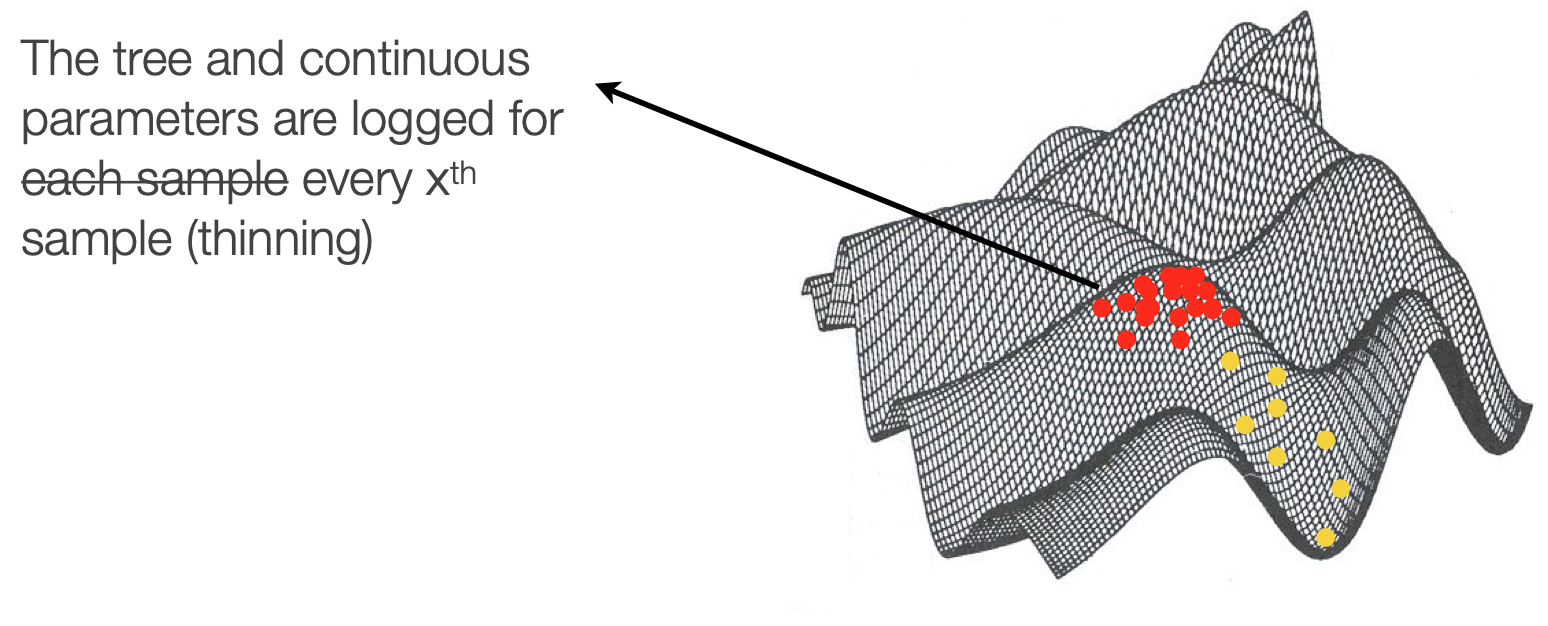
Downsampling
We downsample chains both because of the correlation between states and because of data storage practicality
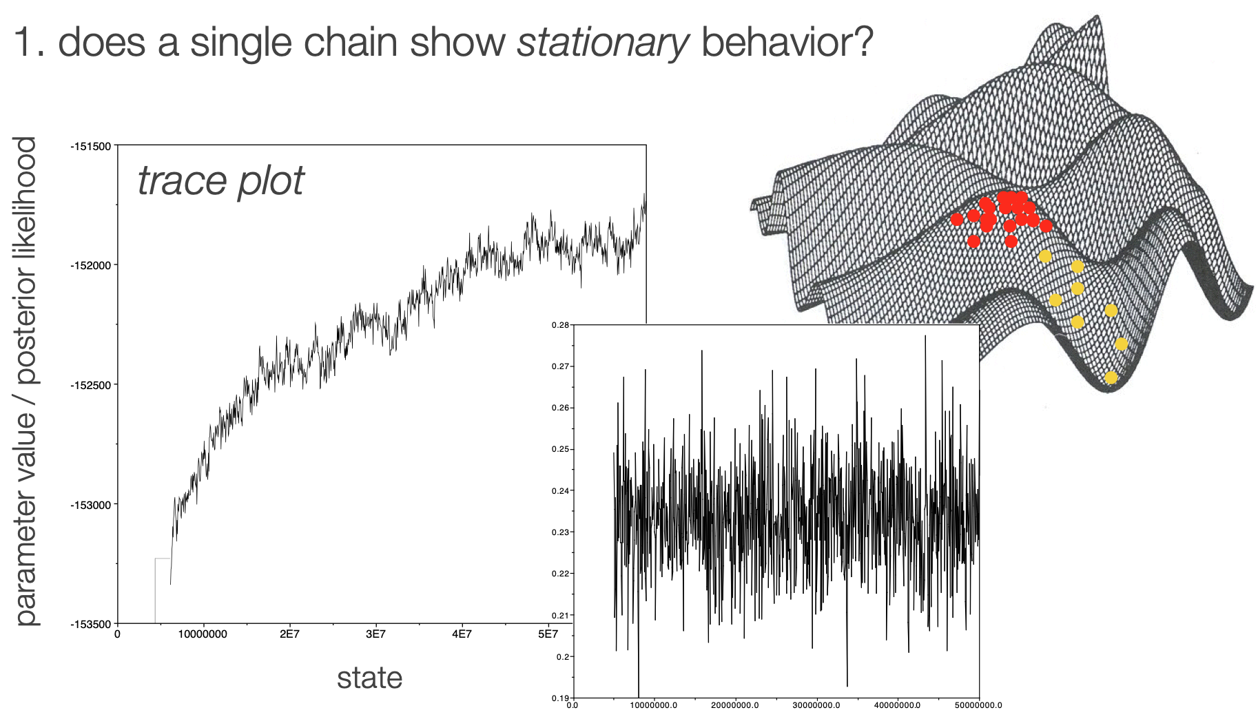
Stationarity
Burn in vs fuzzy caterpillar
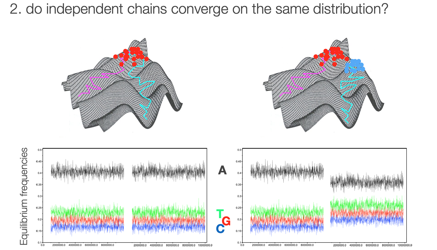
Multiple chains help us determine if we've reached a local or global optimum
Convergence in multiple chains
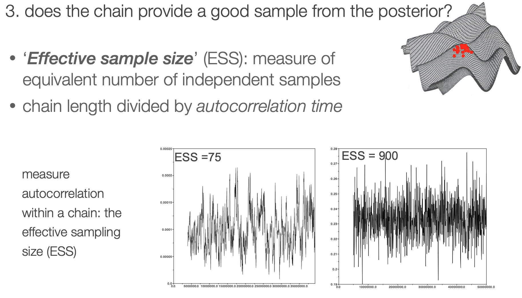
Effective sample size
It is helpful to have an objective statistic for measuring how well the chain represents the posterior
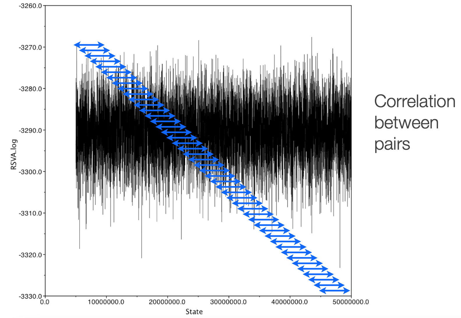
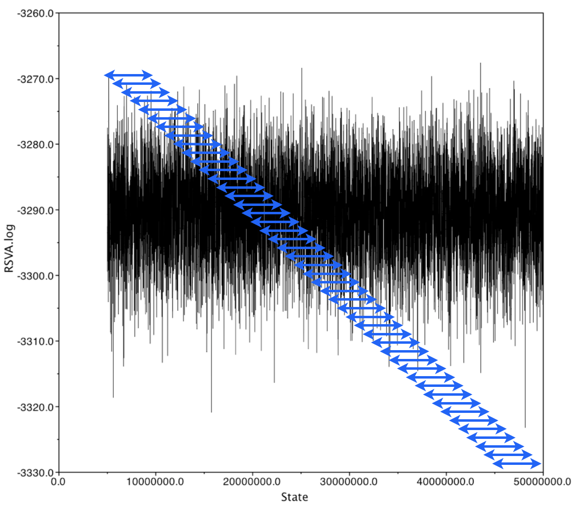
Autocorrelation within a chain
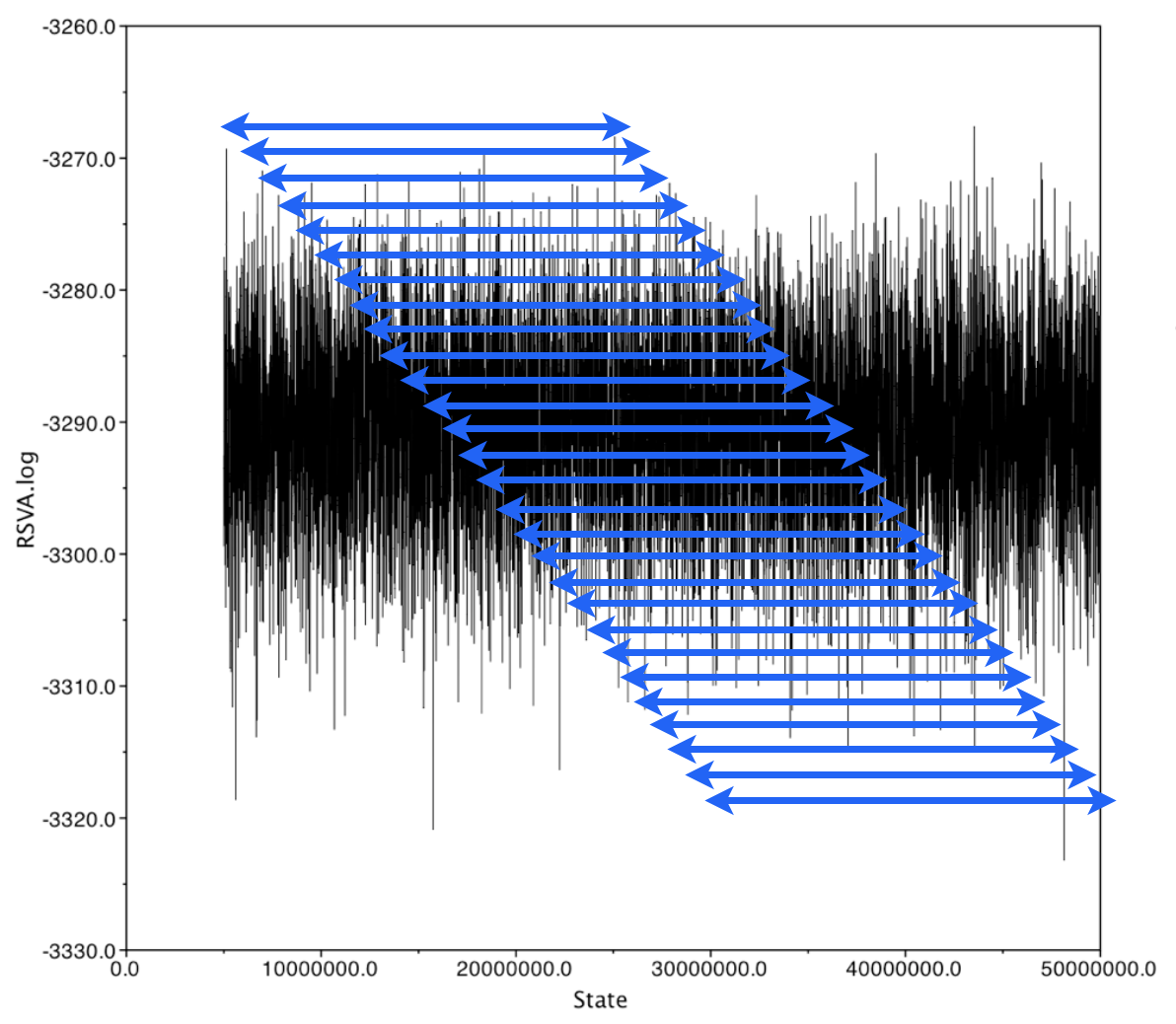
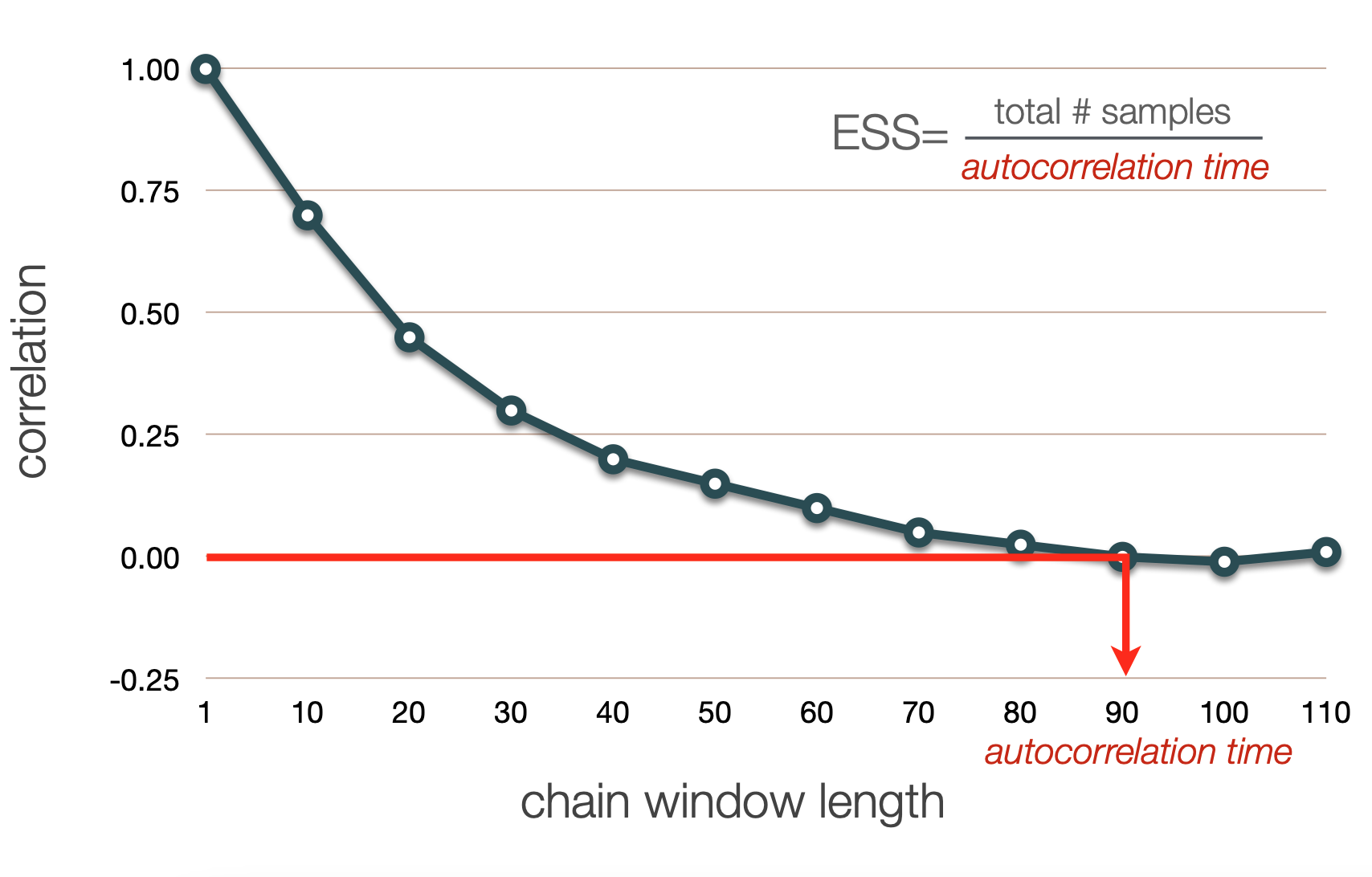
Autocorrelation in a chain is calculated using a "sliding window" approach, where values of the chain are compared across a window of a fixed length. This gets repeated across the whole chain.
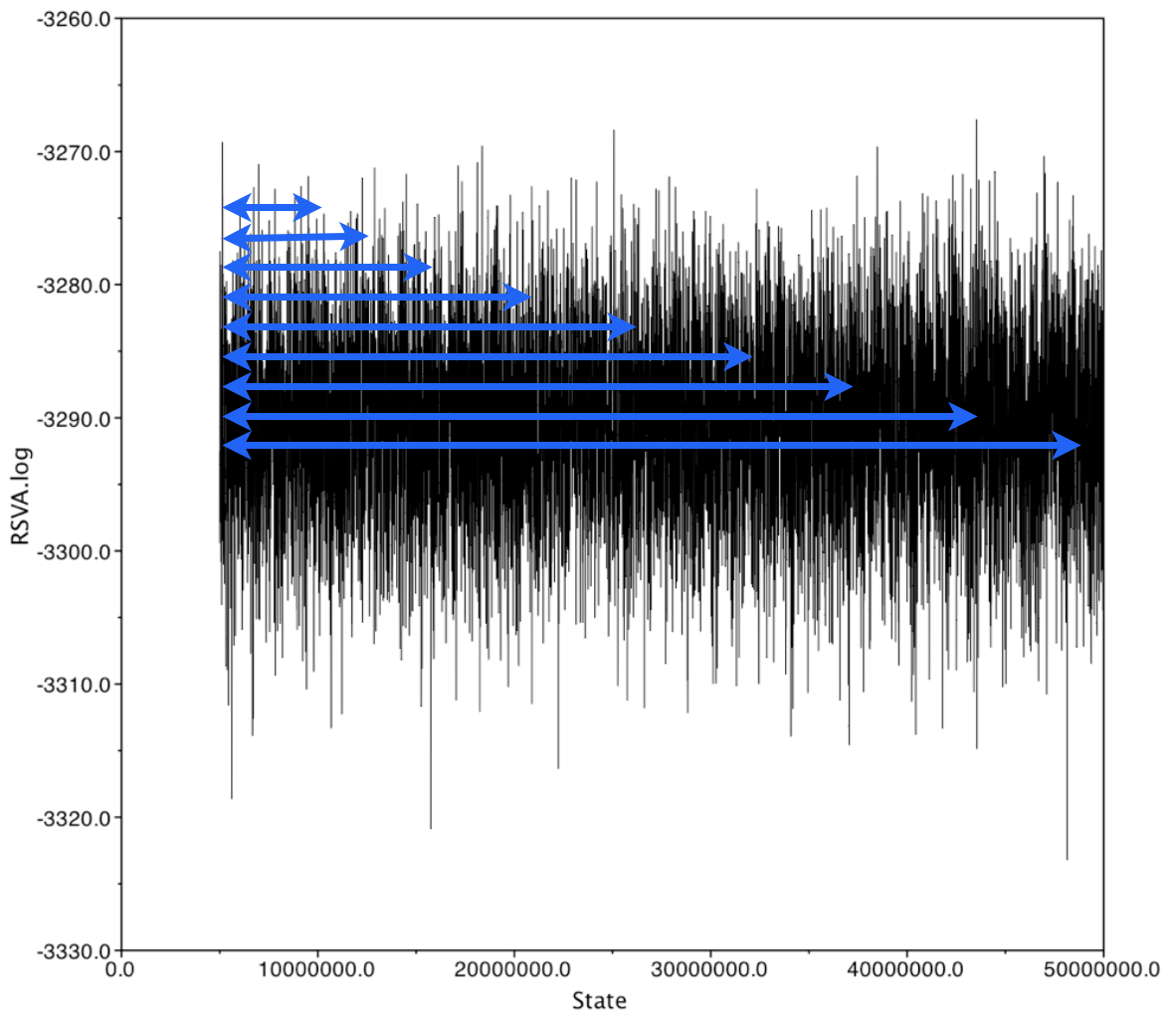
Autocorrelation in the chain can be measured using windows of varying widths
ESS Calculation
Recall: we thin chains because two adjacent samples are extremely correlated
In general, we expect an inverse correlation between chain window lengh and degree of correlation
We can define the chain window length for which the autocorrelation drops below a given threshold as the "autocorrelation time"
ESS is calculated as total/a.c.t.
How do we summarize and interpret the results of our Bayesian phylogenetic analysis?
Summary of continuous parameters
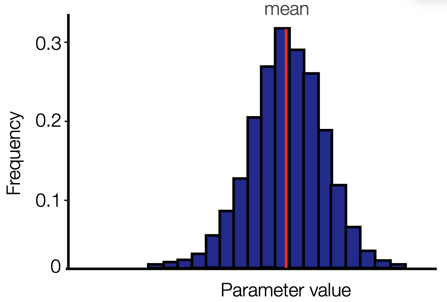
For a well mixed chain we see that most of the samples (shown by density) lie closer to the mean and fewer are further away
We can imagine looking at this chain sideways and "collapsing" it
Posterior distribution
When we do this, we get a posterior probability distribution for the parameter. The mean will often be close to the MLE estimate, but we also get a full distribution
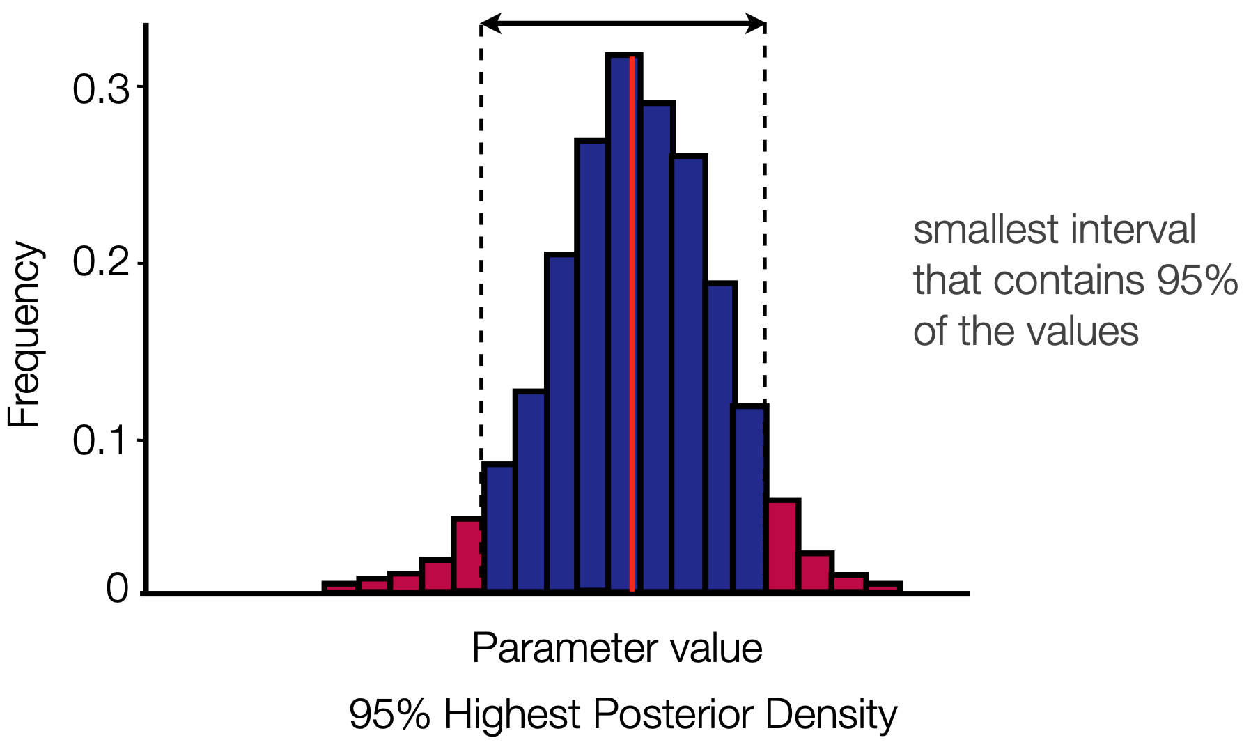
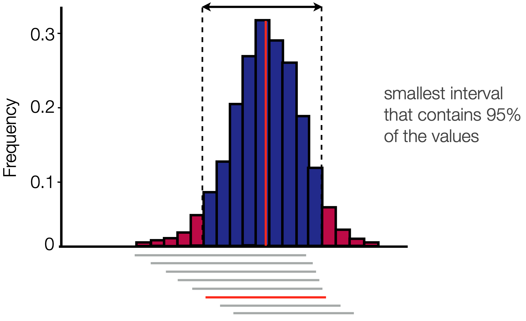
Credible intervals
We usually report not only the parameter mean, but also the 95% HPD
Credible intervals
This is once again calculated using a sliding window approach
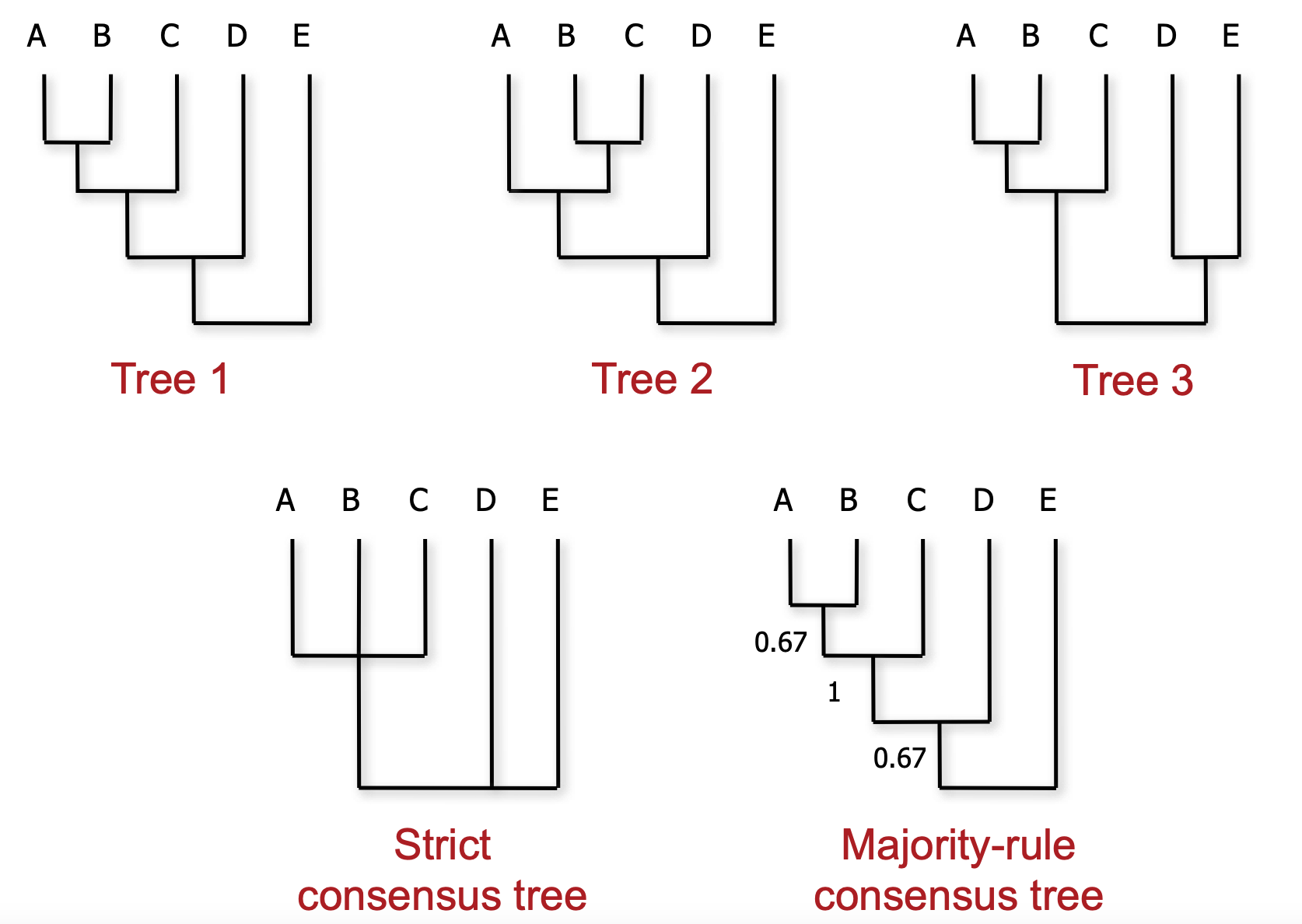
We've discussed how to summarize continuous parameters, however we also want a way to summarize a posterior distribusion of many discrete trees.
How do we choose a consensus?
There are many ways of generating a consensus tree from a sample, with each having its own pros and cons.
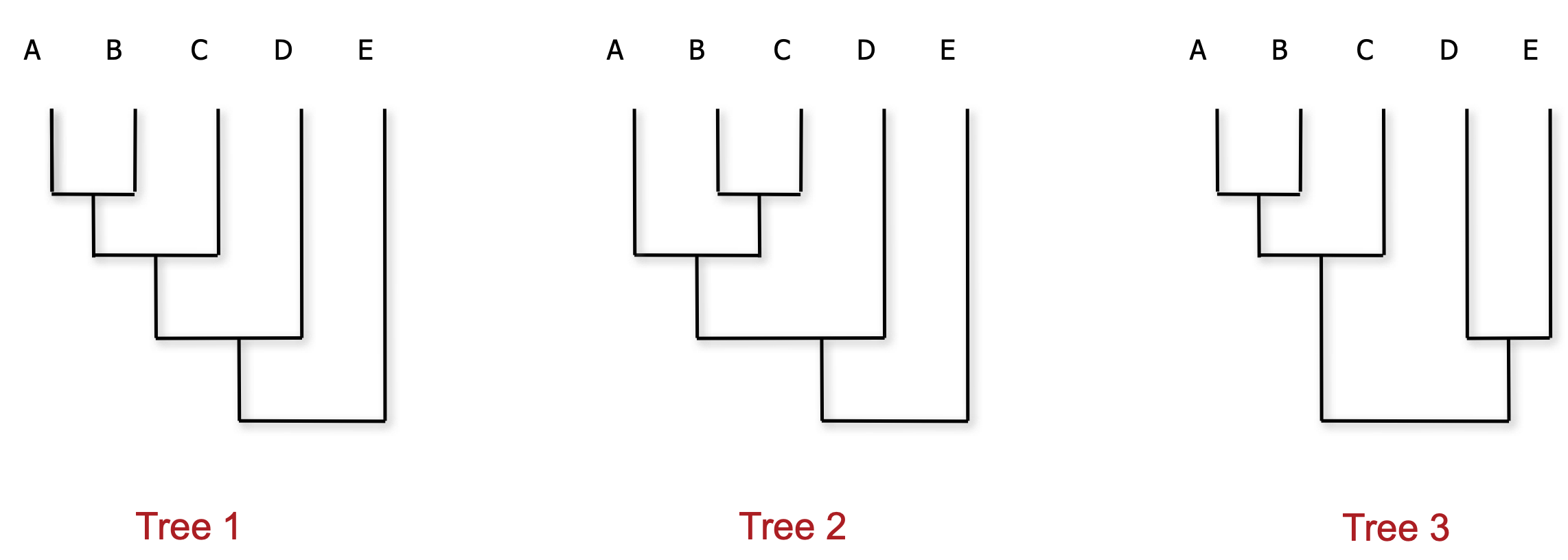
Maximum clade credibility (MCC) trees
We frequently use MCC trees to represent a posterior distribution
MCC tree is a tree from the posterior that best represents the posterior (kind of like a mean)
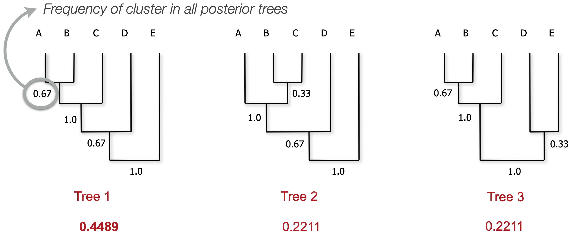
MCC calculation
We consider each clade (monophyletic subtree) that we observe
Calculate the proportion of posterior trees that clade appears in
We then take the product of all clade frequencies for all trees
The tree with the highest score is the MCC tree
My chain won't converge and I am confused and angry and a little bit scared. What can I do?
In the course of running Bayesian phylogenetic analyses we are frequently frustrated by slow convergence and poor mixing.
Some things might help:
Wait; run more parallel chains (different seeds)
Retune parameters (target $10 \text{--} 70\%$ acceptance)
Propose changes to "difficult" parameters more often (operator weights)
Use different operators
Simplify or make the model more realistic (stronger priors)
For this class we will focus on the first, but in research phylogenetics we have many tools in our toolbelt

